

Pivot Tables for Civil Engineers (Part 1)
Introduction
Pivot tables are a super useful tool in Excel that lets you cross tablulate and summarize large datasets. In this article, I’ll go through a tutorial showing some of the basics of Pivot Tables using some sample traffic crash data.
This post is the first post in a multi-part series I’m doing on Pivot Tables. In this post, I’ll show how to make the most basic PivotTable, one that calculates the number of rows in a table.
Sample data
The sample data I’ll use in this tutorial is traffic crash data. An Excel file contains the crash data, and each row represents a crash.
Open the accordion below if you want some more details of the fields in the sample data. The fields in this crash data are very similar to the fields you’ll see in many states’ crash data.
Sample fields
Crash ID:
A unique ID per crash.
Crash Year:
The year the crash occured.
Crash Severity
The following crash severities are used through most of the USA:
- K = A crash with one or more fatalities
- A = A crash with a major injury (generally, one where an ambulance was required), but no fatalities.
- B = A crash with a minor, but visible injury (no ambulance was needed)
- C = A crash with a possible or non-visible injury
- O = A crash with no injuries, but with property damage (also known as a PDO crash)
Persons Injured:
The count of the number of persons injured in the crash.
Vehicles:
The number of vehicles involved in the crash.
Collision Type:
The type of collision that occured.
Jurisdiction:
The city/town/county where the crash isFunctionOrConstructorTypeNode.
All other fields are True/False fields where 1 = the condition occured in the crash and 0 = the condition did not occur for that crash.
The sample excel file has 466 crashes.
The simplest pivot table
To start, we will create the simplest pivot table possible, one which counts the number of records.
-
Open the crash data spreadsheet.
-
To create the pivot table, select all the data in the worksheet.
-
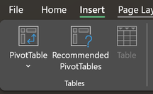
Go to the Insert tab and press the PivotTable button.
-
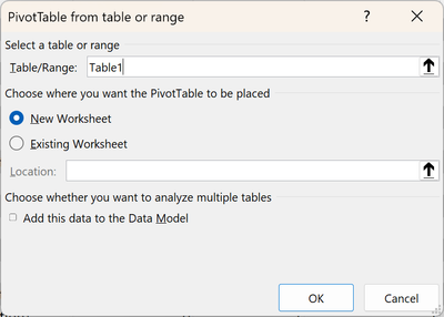
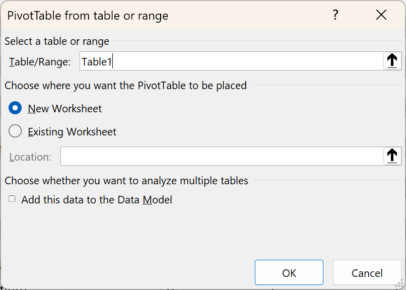
In the dialog that pops up, you can set if you want the PivotTable to show up on a new worksheet or on an existing worksheet. For this tutorial, keep “New Worksheet” checked.
-
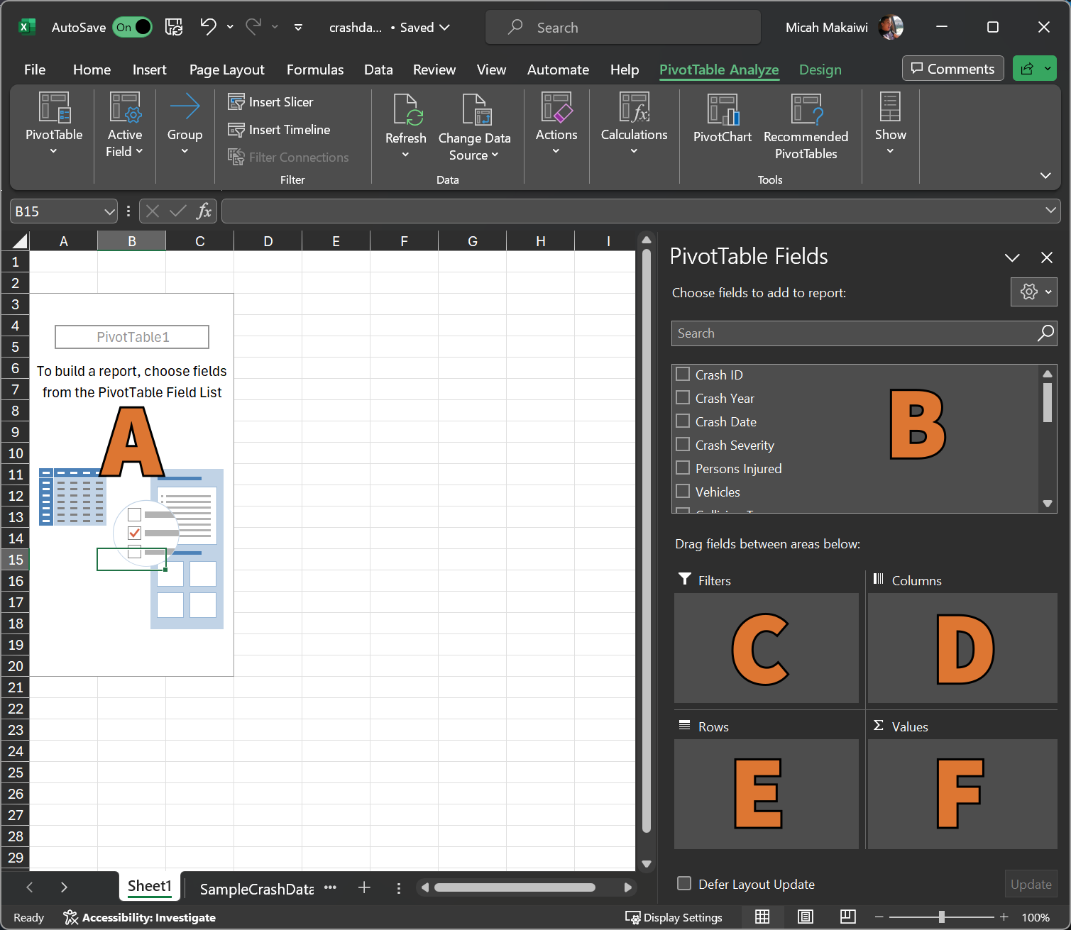
You’ll see a screen like the following:

The screenshot above has the following items of note, labelled 1 through 6.
-
This is your PivotTable. As you build it, your results will show here.
-
This is the list of fields in the source data. You can drag them tothe areas at the bottom (labelled 3 through 4).
-
Drag a field to this area to use that field as a filter for the PivotTable.
-
Drag a field to this area to use that field for your table columns
-
Drag a field to this ara to use that field for your table rows.
-
Drag a field here to use that field for the values in the table.
-
-
For this simple PivotTable, we’ll just count the number of records in the source data. Start by dragging the Crash ID field from the top area (B) to the Values area (F).
-
You’ll see something like the image below. The table has 466 rows, but the result is 108,881. What’s going on?
If you take a closer look, you’ll see that under the Values Section, the field you just dragged is called “Sum of Crash ID.” Excel is taking the Crash ID for each row and summing them instead of just counting them. It’s pretty easy to change this.
-
Click on the arrow to the right of “Sum of Crash ID” and choose Value Field Settings.
-
In the dialog that pops up, select Count. This will count t

Stay tuned for the next part where I’ll show you how to filter a PivotTable.